星期一, 12月 02, 2019

IQA - Image Quality Accessment


https://zhuanlan.zhihu.com/p/32553977


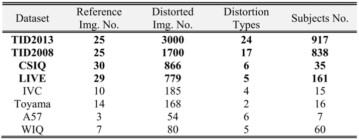
图像质量评价的数据库很多,各种失真类型针对各种图像,但公认度最高的还是前四个,即LIVE, CSIQ, TID2008和TID2013,这些库都提供了每幅失真图像的主观评分值MOS,也就是ground truth。原始图像数量都差不多,前两个库都是针对常见失真类型为主,即加性高斯白噪声、高斯模糊、JPEG压缩和JPEG2000压缩,而TID2013包含失真图像数量有3000幅,主观实验打分人数是917人,权威性当然是最高的,但由于失真类型数量高达25种,同时也是最难的。LIVE和CSIQ两个库可以做到很高了,目前FR IQA的主要战场是TID的两个库(BIQA还是只能在LIVE和CSIQ上玩玩,TID就惨不忍睹了)。下面两个表分别是数据库大致情况,和分别包括的失真类型,这里提到失真类型,是因为后面要用到。
https://xialeiliu.github.io/RankIQA/

https://live.ece.utexas.edu/research/quality/subjective.htm

H.R. Sheikh, M.F. Sabir and A.C. Bovik, "A statistical evaluation of recent full reference image quality assessment algorithms", IEEE Transactions on Image Processing, vol. 15, no. 11, pp. 3440-3451, Nov. 2006.

SSIM

Z. Wang, A.C. Bovik, H.R. Sheikh and E.P. Simoncelli, "Image quality assessment: from error visibility to structural similarity," IEEE Transactions on Image Processing , vol.13, no.4, pp. 600- 612, April 2004.

星期日, 9月 22, 2019

Deep Compression: Compressing Deep Neural Networks with Pruning, Trained Quantization and Huffman Coding


這是一種 DNN model reduction (compression) 的方法:第一個stage 將原有model 中
weight 小於某個threshold 的connection 去除(減斷),並進行重新的training ( 以確保
error rate 沒有增加);第二個 stage 將 network 中每一層的weights 做分群並將各群的中
心(or 平均值)做為 code book 來表示每一層的 weights ( 此步驟 很像 vector
quantization ); 第三個 stage 則是依據 code book 中 code words 出現的機率大小,以
Huffman code 壓缩之。
大部分的 DNN 可壓個 20 倍,執行速度也比較快!(35x to 49x compression ratio was
reported in literature, as expected, this approach is very time and computing
resources consuming in the training phase)。

https://arxiv.org/abs/1510.00149

【深度神经网络压缩】Deep Compression (ICLR2016 Best Paper)
https://zhuanlan.zhihu.com/p/21574328


Neural networks are both computationally intensive and memory intensive, making
them difficult to deploy on embedded systems with limited hardware resources. To
address this limitation, we introduce “deep compression”, a three stage pipeline:
pruning, trained quantization and Huffman coding, that work together to reduce
the storage requirement of neural networks by 35× to 49× without affecting their
accuracy. Our method first prunes the network by learning only the important
connections. Next, we quantize the weights to enforce weight sharing, finally, we
apply Huffman coding. After the first two steps we retrain the network to fine
tune the remaining connections and the quantized centroids. Pruning, reduces the
number of connections by 9× to 13×; Quantization then reduces the number of
bits that represent each connection from 32 to 5. On the ImageNet dataset, our
method reduced the storage required by AlexNet by 35×, from 240MB to 6.9MB,
without loss of accuracy. Our method reduced the size of VGG-16 by 49× from
552MB to 11.3MB, again with no loss of accuracy. This allows fitting the model
into on-chip SRAM cache rather than off-chip DRAM memory. Our compression
method also facilitates the use of complex neural networks in mobile applications
where application size and download bandwidth are constrained. Benchmarked on
CPU, GPU and mobile GPU, compressed network has 3× to 4× layerwise speedup
and 3× to 7× better energy efficiency.

星期五, 9月 20, 2019

DeepN-JPEG: A Deep Neural Network Favorable JPEG-based Image Compression Framework


The marriage of big data and deep learning leads to the great success of artificial intelligence, but it also raises new challenges in data communication, storage and computation [7] incurred by the growing amount of distributed data and the increasing DNN model size. For resource-constrained IoT applications, while recent researches have been conducted [8, 9] to handle the computation and memory-intensive DNN workloads in an energy efficient manner, there lack efficient solutions to reduce the power-hungry data offloading and storage on terminal devices like edge sensors, especially in face of the stringent constraints on communication bandwidth, energy and hardware resources. Recent studies show that the latencies to upload a JPEG-compressed input image (i.e. 152KB) for a single inference of a popular CNN–“AlexNet” via stable wireless connections with 3G (870ms), LTE (180ms) and Wi-Fi (95ms), can exceed that of DNN computation (6∼82ms) by a mobile or cloud-GPU [10]. Moreover, the communication energy is comparable with the associated DNN computation energy.

Existing image compression frameworks (such as JPEG) can compress data aggressively, but they are often optimized for the Human-Visual System (HVS) or human’s perceived image quality, which can lead to unacceptable DNN accuracy degradation at higher compression ratios (CR) and thus significantly harm the quality of intelligent services. As shown later, testing a well-trained AlexNet using CR =∼ 5× compressed JPEG images (w.r.t. CR = 1× high quality images ), can lead to ∼ 9% image recognition accuracy reduction for the large scale dataset— ImageNet, almost offsetting the improvement brought by more complex DNN topology, i.e. from AlexNet to GoogLeNet (8 layers, 724M MACs v.s. 22 layers, 1.43G MACs) [11, 12]. This prompts the need of developing an DNN-favorable deep compression framework.

DeepN-JPEG: A Deep Neural Network Favorable JPEG-based Image Compression Framework
https://arxiv.org/pdf/1803.05788.pdf


Feature Distillation: DNN-Oriented JPEG Compression Against Adversarial Examples
https://arxiv.org/pdf/1803.05787.pdf

Data Science and Engineering


Data Science : Challenges and Directions
Prof. Longbing Cao, Communications ACM, Aug. 2017
http://203.170.84.89/~idawis33/DataScienceLab/publication/DS_CACM.pdf


星期日, 8月 11, 2019

Convolution Theorem and Overlap Save/Add Method


https://github.com/chenhsiu/remagic/blob/master/convolution.ipynb

The Overlap add/save method gives us an idea about how to use FFT to accelerate convolution. This method is generally much faster than typical pair-wise multiplication convolution by its definition. But how many performance gain we can get from this kind of FFT accelerated convolution? Let's do some experiments on the 2D convolution and see its result.


Convolution Theorem

First of all, let's try prove the convolution theorem with the python code.

From time domain

In [32]:
import numpy as np
from scipy.fftpack import fft, ifft, fftn, ifftn

x = [0, 0, 3, -1, 0]
h = [1, 1, 2, 1, 1]

X = fft(x)
H = fft(h)
r1 = np.real(ifft(X*H))

r2 = np.convolve(np.hstack((x[1:],x)), h, mode='valid')
print('%s == %s ? %s' % (r1, r2, 'Yes' if np.allclose(r1, r2) else 'No'))
[1. 2. 2. 2. 5.] == [1 2 2 2 5] ? Yes

From frequency domain

In [31]:
# frequency domain
X = np.array([1.+1.j, 2.+3.j, 1.+2.j, 3.+2.j])
H = np.array([2.+3.j, 1.+1.j, 3.+3.j, 4.+5.j])

Y = X * H
r1 = ifft(Y)
print('r1 = %s' % r1)

x = ifft(X)
h = ifft(H)
x = np.hstack((x[1:], x)) # by default is linear convolution, make it circular
r2 = np.convolve(x,h, mode='valid')
print('r2 = %s' % r2)

print('r1 == r2 ? %s' % ('Yes' if np.allclose(r1, r2) else 'No'))
r1 = [-0.75+10.5j   5.   -1.75j -1.25 -3.5j  -4.   -0.25j]
r2 = [-0.75+10.5j   5.   -1.75j -1.25 -3.5j  -4.   -0.25j]
r1 == r2 ? Yes

Time domain with different size signal

In [16]:
x = [7, 2, 3, -1, 0, -3, 5, 6]
h = [1, 2, -1]

X = fft(x)
H = fft(h, len(x))
r1 = ifft(X * H)
print('r1 = %s' % r1)
r2 = np.real(np.convolve(np.hstack((x[1:],x)),h,mode='valid'))
r2 = r2[len(r2) - len(x):]
print('r2 = %s' % r2)

print('r1 == r2 ? %s' % ('Yes' if np.allclose(r1, r2) else 'No'))
r1 = [ 1.40000000e+01+0.0000000e+00j  1.00000000e+01-2.2977602e-16j
 -1.11022302e-15+0.0000000e+00j  3.00000000e+00+2.2977602e-16j
 -5.00000000e+00+0.0000000e+00j -2.00000000e+00+6.5840240e-16j
 -1.00000000e+00+0.0000000e+00j  1.90000000e+01-6.5840240e-16j]
r2 = [14 10  0  3 -5 -2 -1 19]
r1 == r2 ? Yes

Fast Convolution with FFT

Now we see how the FFT can help us on fast convolution.
The convolve2d in scipy.signal uses pair-wised multiplication (see the source code ). Meanwhile, there is also a fftconvolve in scipy.signal which uses FFT to calculate convolution (see source code here). From its documentation:
This is generally much faster than convolve for large arrays (n > ~500), but can be slower when only a few output values are needed, and can only output float arrays (int or object array inputs will be cast to float).
For overlapadd2, we found a 2D overlap-add with FFT implementation on github. Below is its description:
Fast two-dimensional linear convolution via the overlap-add method. The overlap-add method is well-suited to convolving a very large array, Amat, with a much smaller filter array, Hmat by breaking the large convolution into many smaller L-sized sub-convolutions, and evaluating these using the FFT. The computational savings over the straightforward two-dimensional convolution via, say, scipy.signal.convolve2d, can be substantial for large Amat and/or Hmat.
The performance comparison result on my NB shows below:
methodconvolve2dfftconvolveoverlapadd2
speed3040 ms30.1 ms94.8 ms
We can see the FFT based convolution is generally much faster than typical convolution, from 30X to 100X acceleration. The result surprises me a bit because fftconvolve is still faster than overlapadd2. The overlapadd2 looks good and ideal, but the user still needs to tweak the size of L in order to get the best performance. Maybe overlapadd2 has the real benefits only when the input matrix is so big that can't be fit into memory and we have split into sub-convolutions.
One thing to note is, when we use FFT convolution on image processing, there will be a dark borders around the image, due to the zero-padding beyond its boundaries. The convolve2d function allows for other types of image boundaries, but is far slower.

Reference

There is an article doing 2D convolution benchmark with various convolution libraries:
In [75]:
# before you run, eval the cell containing overlapadd2 at the end

from scipy import misc
import scipy.signal as sp
import matplotlib.pyplot as plt

A = misc.ascent()
A = A.astype(float)
print(A.shape)
H = np.outer(sp.gaussian(64, 8), sp.gaussian(64, 8))

print('==> using convolve2d')
%time B1 = sp.convolve2d(A, H, mode='same')
print('==> using fftconvolve')
%time B2 = sp.fftconvolve(A, H, mode='same')
print('==> using overlapadd2')
%time B3 = overlapadd2(A, H)

fig, (ax_orig, ax_conv, ax_fft2conv, ax_ovadd2) = plt.subplots(1, 4, figsize = (12, 8))
ax_orig.imshow(A, cmap='gray')
ax_orig.set_title('Original')
ax_orig.set_axis_off()
ax_conv.imshow(B1, cmap='gray')
ax_conv.set_title('convolve2d')
ax_conv.set_axis_off()
ax_fft2conv.imshow(B2, cmap='gray')
ax_fft2conv.set_title('fftconvolve')
ax_fft2conv.set_axis_off()
ax_ovadd2.imshow(B3, cmap='gray')
ax_ovadd2.set_title('overlapadd2')
ax_ovadd2.set_axis_off()
fig.show()
(512, 512)
==> using convolve2d
CPU times: user 2.84 s, sys: 4.87 ms, total: 2.84 s
Wall time: 2.84 s
==> using fftconvolve
CPU times: user 28.4 ms, sys: 11 µs, total: 28.4 ms
Wall time: 28.8 ms
==> using overlapadd2
L = [288 288]
Nfft = [360 360]
CPU times: user 54 ms, sys: 1.89 ms, total: 55.9 ms
Wall time: 56.1 ms
/usr/local/lib/python3.7/site-packages/ipykernel_launcher.py:32: UserWarning: Matplotlib is currently using module://ipykernel.pylab.backend_inline, which is a non-GUI backend, so cannot show the figure.

lec-1 (2022-05-12) Accelerating deep learning computation & strategies

雖然用 DNN train/predict model 也好一陣子了,但這週才是第一次搞懂 cuDNN 是作什麼的 以前好奇過 tensorflow/pytorch 是怎麼做 convolution 的,FFT 不是比較好嗎? 下面的 reference 就給了很好的解釋: Wh...